
Extremes
JM Coastal can carry out extreme value analysis of observed and hindcast water level and wave data. This can be combined with Monte Carlo simulations to create thousands of years of data that can be input into coastal flood simulations to provide in-depth flood risk analysis and input in to coastal defence design.
The expected frequency of a coastal flood is often described by the return period (e.g. 1 in 100 years). Coastal defences are also often designed to prevent significant flooding for a certain return period that relates to the nearshore water level and/or wave conditions. However, different combinations of water levels and wave heights can combine to give the same return period but lead to different levels of coastal flooding. Therefore, to carry out a rigorous coastal flood risk assessment along a particular stretch of coast, the joint probability of particular water levels occurring at the same time as certain wave heights should be investigated. Extreme water levels and wave heights also usually exhibit a partial dependence (both are driven by the same storm) and therefore their correlation must also be taken into account.
Case study - Coastal flooding in New Brighton
Due to its location in the Eastern Irish Sea, New Brighton is affected by a large tidal range with potential storm surges and large waves. Although the town is protected by coastal defences such as the King's Parade Sea wall and breakwaters, the combination of high water levels and waves has led to significant coastal flooding, most notably in December 2013 1Wadey M., Brown J., Haigh I. & Dolphin T. Assessment and comparison of extreme sea levels and waves during the 2013/2014 storm season in two UK coastal regions. Nat. Hazards Earth Syst. Sci. 15, 2209–2225 (2015).. On 5th December 2013 flooding caused significant disruption and the council carried out a flood investigation report 2Flood investigation report for December 5th 2013.. In this case study an investigation of flood risk due to the combination of high water levels and waves was carried out using water level data from the tide gauge at Liverpool and the Liverpool bay WaveNet buoy. Return periods for extreme sea level were determined using the Skew Surge Joint Probability Method 3Batstone C. et al. A UK best-practice approach for extreme sea-level analysis along complex topographic coastlines. Ocean Eng. 71, 28–39 (2013).. Generalised Pareto distributions (GPD) were fitted to a subset of the most extreme wave heights and skew surges using a maximum likelihood estimator (MLE) to determine the extreme tails of their distributions. A long term Monte-Carlo simulation (2000 years) that randomly samples the marginal and empirical or fitted (Weibull) distributions of water levels and wave heights taking into account their correlation was then carried out 4Hawkes P.J. et al. The joint probability of waves and water levels in coastal engineering design.
Journal of Hydraulic Research. 40, 241-251 (2002).. The return period of the various combinations of water levels and wave heights could then be determined. Coastal flood simulations were then carried out for 8 samples of combined water levels and wave heights with a joint probability return period of 100 years.
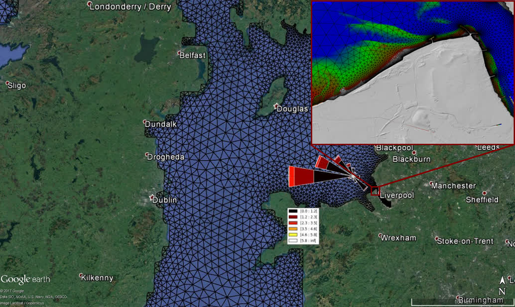
An offshore model system is used to simulate the development of the tide and storm surge in the Irish Sea (Telemac-2D). A high resolution nearshore modelling system (Telemac-2D coupled with Tomawac) that couples the tide and surge with the waves is then used to simulate water levels and wave heights right up to the defence line. Only waves propagating from the west were simulated in this experiment which is the dominant wave direction in the Eastern Irish Sea as shown by the wave rose in the figure above. At the defence line overflow and wave overtopping rates were calculated using equations detailed in the Eurotop manual 5EurOtop - Manual on wave overtopping of sea defences and related structures. and used as boundary conditions to an inundation model (Flood Modeller) using a 5 m resolution grid aggregated from 1m lidar data from the EA open survey data.
ⓘ Figure information
1. The red dots show observed water levels and wave heights - hover on the larger events for more information.
2. The blue lines are contours of equal joint return period for the observed and simulated water levels and wave heights.
3. The green dots are samples from the joint 100 year return period water level and wave height - click on the green dots to see the resultant flooding in the Google Earth image. Refresh the page if they are not visible.